
Scope guide · History & 3D
3D Histogram
Extend component populations into a rolling 15-second waterfall.
ProfessionalLearn & Reference / Scope library / 3D Histogram
How has the distribution changed over time?
Add this view from Add scope > 3D Histogram, then choose the input you want to inspect. Use the pane's i button for its in-app reading guide.
Read this example.
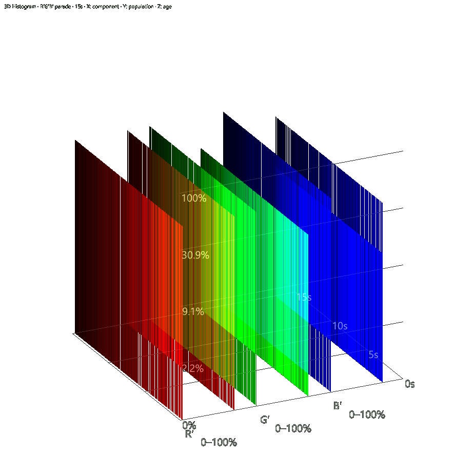
- R′, G′ and B′ panels separate components; position across each panel is level.
- Bar height is sampled population. Logarithmic labels make smaller populations easier to compare.
- Age runs through depth to the 0s front edge. Repeated distributions form repeated layers.
Try it yourself.
- Open from Add scope or the Histogram cube icon.
- Choose a component; compare Overlay and Tiled.
- Rotate to read age, then compare linear and logarithmic Count scale.
Useful controls.
- Uses the standard Histogram catalog, including HSV.
- A fixed 0–100% population scale relates height to each component’s sampled total.
- Up to ten distributions per second retain 15 seconds; Freeze and Clear history support inspection.
Changing source, component or count scale starts a fresh history.